Study Paths, Riemann Surfaces, and Strebel Differentials
Peter Buser
École Polytechnique Fédérale de Lausanne, Switzerland
peter.buser@epfl.ch
Klaus-Dieter Semmler
École Polytechnique Fédérale de Lausanne, Switzerland
This paper is dedicated to the memory of Mika Seppälä and to Cici Safkan-Seppälä
ABSTRACT. These pages aim to explain and interpret why the late Mika Seppälä, a conformal geometer, proposed to model student study behaviour using concepts from conformal geometry, such as Riemann surfaces and Strebel differentials. Over many years Mika Seppälä taught online calculus courses to students at Florida State University in the United States, as well as students at the University of Helsinki in Finland. Based on the click log data of his students in both populations, he monitored this course using edge-decorated graphs, which he gradually improved over the years. To enhance this representation even further, he suggested using tools and geometric intuition from Riemann surface theory. He also was inspired by the much-envied Finnish school system. Bringing these two sources of inspiration together resulted in a promising new representation model for course monitoring. Even though the authors have not been directly involved in Mika Seppälä’s courses, being conformal geometers themselves, they attempt to shed some light on his proposed approach.
Keywords: Study paths, Riemann surfaces, conformal geometry
ISSN 1929-7750 (online). The Journal of Learning Analytics works under a Creative Commons License, Attribution - NonCommercial-NoDerivs 3.0 Unported (CC BY-NC-ND 3.0)
(2017). Study paths, Riemann surfaces, and Strebel Differentials. Journal of Learning Analytics, 4(2), 62–75. http://dx.doi.org/10.18608/jla.2017.42.7
1 INTRODUCTION
This paper illustrates a concept in learning analytics with a strong mathematical component. In particular, it makes use of terms such as “Riemann surfaces” and “quadratic differentials,” which are certainly new to most learning analytics practitioners. Aware of this, we have tried to avoid mathematical jargon, definitions, and theorems, while “demystifying” the crucial technical terms using illustrative figures. We shall, however, start out as though this was a math paper to overview where the ideas come from. The necessary explanations will be provided later in the text.
Strebel’s (1984) theorem asserts that any Riemann surface may be viewed as a collection of Euclidean rectangles that have been pasted together according to some bifurcation data. This structure appealed to Mika Seppälä because surfaces constructed in this way are not only able to capture all the information stored in edge-decorated graphs as used for course monitoring but also make it possible to follow up study paths of individual students or student groups. His aim was twofold:
- To collect experience data to improve the course, add helpful resources, and diagnose shortcomings of the course structure.
- To help students during the course if, in comparison with experience data, their study paths reveal an immanent failure.
In his own words, Seppälä (2014a) put it this way: “The goal [is to build] recommendation systems that advise individual students based on the log data of a large number of past students and on personal characteristics of the student in question.”
To explain concisely the way this is envisaged, we use as an example an aspect of the Finnish school system (Hancock, 2011). In primary and secondary school in Finland, frequent short diagnostic tests are applied throughout the school year to react to gaps in student progress. These tests bifurcate students to different paths of activities and resources with the aim of helping them reach the end of the program successfully. The idea is that all students should get through the year successfully and the activities continue smoothly into the next school year.
The diagram in Figure 1 shows this schematically in a graph. The dots are the vertices of the graph and the lines are its edges. Each vertex represents an event at which students are diagnosed. The edges leaving a vertex to the right represent the different variants of the program of activities that follow the test. According to the outcome of the test, a student is assigned to one of these. All students reach the next test but not necessarily along the same path.

Figure 1: Schematic diagram for study pathways in the Finnish school system.
This contrasts with the diagram in Figure 2, schematizing the approach of still many a contemporary central European school system: bifurcating the students only at the end of the school year into two groups — “promoted” and the dreadful “held back,” which implies repeating the school year and following the same program once more.

Figure 2: Bifurcation at the end of the year into “promoted” and “held back.”
Diagrams such as these are more instructive when decorated by data. One may, for instance, attach to an edge the relative percentage of students currently following it or who have followed it over a particular period of time. For monitoring purposes, however, if advice is intended to be given to individual students, decoration is not always useful. One seeks, therefore, to replace graphs as a form of graphical representation by higher dimensional objects — for instance surfaces. Figure 3 shows such a surface obtained by “thickening” part of the graph in Figure 1. In this thickening process, it is the surface of the solid object that will be retained for the representation.

Figure 3: Thickening of a graph into a surface. The trajectory on the right represents a possible study path that may be chosen by a student.
Mika Seppälä’s proposition for a new type of model was to define the thickened graphs explicitly as Riemann surfaces and the possible study paths on it as trajectories of Strebel differentials. In the following sections, we interpret this approach using the videos of Seppälä (2013, 2014a, 2014b) as underlying references.
Although the model is intended to be used for online courses with many diagnostic events and occasionally high degrees of bifurcation, we shall use school systems to illustrate the concepts, as they are familiar and simple.
2 RECTANGLES AND CYLINDERS
An edge of a graph is essentially the same as a straight-line segment, and the simplest way of “thickening” it is to replace it by a Euclidean rectangle that has both length and width. On any rectangle, we have two (perpendicular) standard foliations formed by the straight lines that are parallel to the sides of the rectangle. We single out the one, called the horizontal foliation, whose lines are in the direction of the edge in which the rectangle is thickening. The other foliation is then called vertical.1 The horizontal lines — we may use any number of them in a rectangle — shall be used to represent parts of oriented study paths of either individual students or student groups with a given study behaviour. On the surface that will be obtained by pasting such rectangles together (see the next section) the horizontal lines merge into global study paths that may be followed over several rectangles.
The second simplest thickening of an edge consists of replacing it by a cylinder. This type of surface may be constructed by pasting together two parallel sides of a rectangle as shown in Figure 4. Think of the rectangle as a sheet of paper, bend or roll it up to bring the two horizontal sides into matching position and then glue them together. In Riemann surface theory, this pasting process is defined without such pictorial description, it suffices to describe, for any point P on the lower side of the rectangle, the corresponding point P′ on the upper side that P would be in contact with after the bending, and then declare the couple {P, P′} as being just one point. In Riemann surface jargon: P and P′ are identified. (The reader who uses a street map in booklet form is confronted with this kind of identification when a street annoyingly leaves on top of the currently open page and then continues on the bottom of some other page.) Figure 4 shows a pair of identified points. P and P′ have the same distance to the left (or the right) vertical side of the rectangle and are thus endpoints of some line L of the vertical foliation.
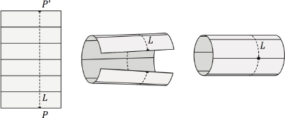
Figure 4: Conformal rectangle with a selection of horizontal leaves folded into a cylinder. The dotted line belongs to the vertical foliation. On the cylinder, it becomes a closed curve.
On the cylinder, L then becomes a closed curve. Hence, the cylinder too carries a horizontal and a vertical foliation. The vertical leaves are closed curves parallel to the two boundaries, the horizontal leaves are the straight lines that go from one boundary to the other. The latter may again be used to represent individual trajectories on a study path.
3 BIFURCATION AND MERGING DATA
A bifurcation arises if decision events direct students into various categories or studies. The bifurcating events may be exams, quizzes, or tests provoking a decision by the teacher, or a decision by students to skip some exercises or learning modules. Merging also takes place commonly in a course or school.
It is difficult to imagine rectangles or cylinders bifurcating, but in Riemann surface theory this is a standard scenario realized via pasting. Figure 5 shows what is called a pair of pants bifurcating from the “waist” cylinder (grey shaded) into the two “leg” cylinders, where the latter are not necessarily of the same widths. On the right hand side, the result of the pasting is again shown in a pictorial way. To this end the cylinders have undergone some deformation in the neighbourhood of the boundary so that they can be brought together into matching position. In Riemann surface theory, such deformations and bringing into matching position are not necessary. It suffices to enumerate the cylinders and list the pasting rules; that is, to indicate which parts of the boundaries of the cylinders to paste together. In Figure 5, for instance, the pasting rule is that any point of the red arc on the boundary of cylinder C1 is identified with a point of the red part on the boundary of C2, any point of the brown arc on C1 with a point of the brown arc on C3, and any point of the green arc on C2 with a point of the green arc on C3. A geometric condition for the pasting is that arcs of the same colour have the same lengths. On the resulting pair of pants these arcs form a triple of arcs that meet in two points. Later on, this triple will be understood as an example of a critical vertical trajectory.
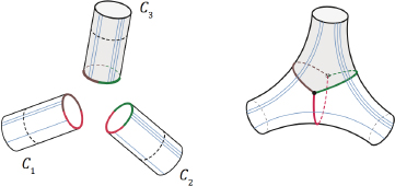
Figure 5: A triple of cylinders pasted together along the boundaries into a surface element called a pair of pants. For visual representation, the cylinders are deformed to match.
Strebel’s (1984) theorem2 states, among other things, that any Riemann surface may be obtained by such pastings. For our purposes, we may thus phrase the following definition: a Riemann surface is an object obtained by pasting together cylinders according to a set of pasting rules.
Because cylinders, in turn, are obtained by pasting together two opposite sides of a Euclidean rectangle, we may, equivalently, say that a Riemann surface is an object obtained by pasting together Euclidean rectangles according to a set of pasting rules.
In the applications to learning analytics, the pasting rules result from bifurcation and merging data. A (much simplified) example common to many central European school systems is the bifurcation at the end of primary school that directs pupils into lower middle and high school. Figure 6 shows the correspondingly pasted cylinders — here we have a waist cylinder and three legs — together with many trajectories indicating the percentage of students in the three study paths. (The 20–30–50 percentages have been chosen for graphical simplicity and are only roughly realistic). The bifurcation data are based on overall past performance. Monitoring is not provided in this model and the surface representation on the left in Figure 6 has no real advantage over the decorated graph on the right. This shall change when monitored courses are looked at. For the learning analytics of the latter, Strebel differentials are interesting as they exhibit the same bifurcation patterns. Let us now outline, at least pictorially, what they are.

Figure 6: Bifurcation at the end of primary school into lower, middle, and high-school. Monitoring and redirecting is not provided in this model.
4 STREBEL DIFFERENTIALS
In complex function theory, a quadratic differential is a mathematical expression that can be written in the following form:

where z is a variable that runs through complex numbers, φ is a complex differentiable function, and 𝑑𝑧 is another complex variable, intended to play the role of a “variation of z.” Geometrically z, dz, and φ(z)dz2 are interpreted as certain points in the Euclidean plane, where the plane is endowed with a cartesian coordinate system. A deeper understanding of the meaning of the expression “φ(z)dz2” will not be necessary for our purposes, it suffices to remark that it leads to patterns such as those in Figures 7–9.
If we draw a straight line from the origin of the coordinate system to z, then this line forms an angle with the first coordinate axis, called the argument of z, denoted by arg{z}. Similarly, dz and φ(z)dz2 have the arguments arg{dz} and arg{φ(z)dz2}. There are rules about how to compute the argument of φ(z)dz2 using complex number calculus.
We may visualize a quadratic differential by a field of straight line segments. To this end, we sort out for any z the particular value of dz that has distance 1 to the origin and satisfies

Figure 7 shows these fields for the functions φ(z) = 1, φ(z) = z, φ(z) = z2 and φ(z) = z4. Each rectangle shows the same part of the Euclidean plane with the origin of the coordinate system in the centre. To obtain the graphical representation, we have selected a number of points spread out in the plane and then drawn for any selected point z a straight-line segment going from z to z + rdz. The additional factor r in this drawing instruction has been chosen to give the line segments a length that makes the field “look good.”

Figure 7: Line fields of quadratic differentials in the plane.
The segments in these figures seem to align along curves. Indeed, one of the results about quadratic differentials is that the entire plane is filled out with a family of smooth curves to which the line segments are tangent. These curves are called the horizontal trajectories of the quadratic differential. Figure 8 shows these trajectories for the preceding examples. In these examples, an exceptional situation is given at point z = 0 (the centres of the squares). Here several trajectories merge. In a situation like this, the merging point is called a critical point and the merging trajectories are called critical trajectories.

Figure 8: Horizontal trajectories of quadratic differentials in the plane.
If we replace the above angle condition for the line field by the condition

all segments of the field become rotated by π/2 that is, by 90 degrees, and we get the foliation of the plane by the so-called vertical trajectories. Horizontal and vertical trajectories intersect each other orthogonally (except at the critical point). Figure 9 shows both foliations together, again for the preceding examples.

Figure 9: Horizontal trajectories (blue) and vertical trajectories (brown) of quadratic differentials in the plane. The straight lines emerging from the centre are the critical trajectories.
In a similar way, quadratic differentials with horizontal and vertical trajectories exist also on Riemann surfaces. Figures 5 and 10 show two cases of a general construction that produces many — albeit not all — such differentials: cylinders with the standard horizontal and vertical foliations are pasted together along their boundaries according to some given pasting rules. The pairs of horizontal and vertical foliations of the cylinders together yield two foliations of the resulting surface, which then again shall be called horizontal and vertical foliations. Part of the aforementioned Strebel theorem states that these foliations are the trajectories of a uniquely determined quadratic differential. The differentials obtained through these constructions are called Strebel differentials.3
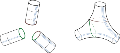
Figure 10: Trajectories of a Strebel differential on a pair of pants. The thin lines (blue) are the horizontal trajectories, the thick self intersecting curve is a critical vertical trajectory and the intersection point is a critical point.
The boundaries of the cylinders pasted together become the critical vertical trajectories on the surface. They consist of arcs that come together at certain points, called the critical points. Part of Strebel’s theorem also states that in the neighbourhood of a critical point on the surface, the trajectories look exactly as the trajectories in the neighbourhood of a critical point of a differential in the plane.
Figures 5 and 10 illustrate this on a pair of pants, drawn as a surface in space. The marked arcs on the boundaries of the cylinders pasted together turn into the arcs of the critical vertical trajectory on the surface; the endpoints of the arcs become the critical points. In the first example, we have two critical points, each with three “arms”; in the second example, there is one critical point with four outgoing arms. The two critical points of the first example correspond to the differential zdz2; the second example corresponds to z2dz2.
Observe how the horizontal trajectories on the surfaces bifurcate at the critical vertical trajectories. Such patterns may be quite involved. Figure 11 shows cases that will be used in the next section.
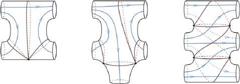
Figure 11: Surface elements with a critical vertical trajectory (brown) and a selection of horizontal trajectories (blue). The critical points with 6 arms in the first two examples corresponds to the last case in Figure 9.
It is through this bifurcation aspect that Mika Seppälä aimed to investigate Strebel differentials as a possible model for the representation of student study paths through monitored online courses.
5 EXAMPLES
Here we illustrate some examples of how certain structural elements of a course or a school system may be illustrated with these methods. We first extract from Seppälä (2013, 2014a, 2014b) the way in which the model based on these methods is intended to be used. The following examples are from our own interpretation.
In the extraction, “resources” means textbooks, lecture notes, videos, solved problems, and so on; “learning characteristics” means a way of using the resources and approaching the exercises of the course; “examination events” means brief or extended diagnostic tests, quizzes, peer graded workshops, instructor graded exams, final examinations, and so on. The following list outlines what the geometric objects described in the preceding sections are intended to represent:
- Cylinder: a proposed package of activities between two examination events
- Critical vertical trajectory: an examination event
- Horizontal trajectory: study path of a hypothetical student with given learning characteristics
- Width of a cylinder: overall percentage of students whose study paths go through that cylinder
- Length of a cylinder: this definition is left to the intended use by the instructor; for example, the duration of the activity
- Monitoring: the instructor’s advice given to the student to improve the predicted learning outcome by switching trajectories (= to modify the learning characteristics)
The first example (Figure 12) shows schematically the procedure in Finnish schools corresponding to the graph in Figure 1. The edges of activities are now replaced by gray shaded cylinders and the examination events are represented by non-shaded surface elements. The critical vertical trajectories are not drawn. Trajectories 1, 2, and 3 correspond to profiles of students who remain at a certain level. Trajectory 4 bifurcates from level two to level three at the test event in the middle and then remains at the same level. Students in trajectory 2 may be encouraged by the instructor to modify their study characteristics so as to switch from trajectory 2 to trajectory 4 that later will be on level three. Other trajectories oscillate between two levels, and so on.
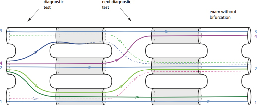
Figure 12: Hypothetical study paths in Finnish schools represented as trajectories of a Strebel differential on a Riemann surface.
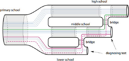
Figure 13: One year bridge programs allowing students who are about to finish lower or middle school to reach middle school or high school graduation.
The same structure may show up in an online course, a student may be directed to a program that offers additional exercises depending on what part of the weekly quiz has been missed. A student may also be encouraged by the instructor to make different use of the resources and thus switch to a trajectory with a better predicted outcome.
The next figure illustrates an improvement over the school system schematized earlier in Figure 6. Many schools offer one year bridge programs (so called passerelles) allowing late bloomers to reach middle or high school. A more complex surface with additional diagnostic tests at the end of the classical program represents this scheme. Representing various categories of learning behaviour by different trajectories and following trajectories backwards, for instance along the red dotted one, may lead to a revision of the decision procedure at the end of primary school.
The final two examples are taken from the École polytechnique fédérale de Lausanne in Switzerland (EPFL, 2016). Figure 14 depicts the promotion system for engineering students in their first two years of study at EPFL as it has been in practise until the academic year 2015–2016. The scheme is represented schematically as a Strebel differential on a Riemann surface. Each grey shaded cylinder represents a one year program consisting of two terms. In the cylinders on the lower level, no educational program such as a possible summer school is foreseen. (For graphical simplicity, the thicknesses of the cylinders do not represent the percentages of students correctly.) A final exam for promotion and relegation takes place at the end of every year. Students in trajectories 1, 2, and 3 reach the third year successfully; students with two successively failed finals must drop out.
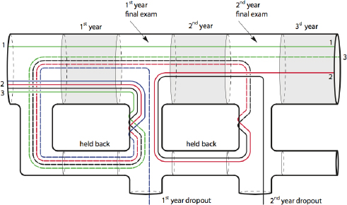
Figure 14: Strebel differential representing relegation and promotion of first and second year engineering studies at EPFL.
EPFL has recently restructured its first-year study plan by inserting a new bifurcation after the first semester, taking out students not likely to make it at the end of the year and putting them into a special program with its own exam during the second semester. It is assumed that this will allow them to restart the first-year program with better preparation. Figure 15 shows the reform effort. To separately track the future progress of students who have followed the special program, we have replaced the surface of Figure 14 with a more complex one.
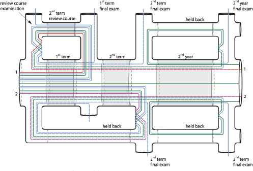
Figure 15: Reform of first-year engineering studies at the EPFL.
Students failing the exam after the first term are required to follow the newly offered full-time review course (cours de mise à niveau) during the second term, at the end of which they must pass a special exam. Students having passed this exam are admitted to a second round of the first-year program. It is expected that students who have followed the review course, such as those in trajectory 1, will have better future performance than those repeating the first year “classically,” such as those in trajectory 2. Replacing the 1st term final exam with a differentiating diagnostic test bifurcating the students into different variants of the review course may further improve this.
6 FINAL REMARKS
As mentioned in the beginning, Mika Seppälä’s motivation for graphical course representation was to improve his online courses and advise students to use well chosen additional resources to ensure success and avoid dropouts. Here are the obvious advantages of a more surface-like representation of student learning characteristics and course data in view of these goals:
The surface representation provides a visual tool to analyze and improve the course structure. In looking at student data recorded by trajectories on a surface, one may locate shortcomings; for instance, by following backwards the trajectory of a student who eventually dropped out. Too difficult exercise sheets, too heavy workloads, and so on at the beginning of the course may have caused an unsuccessful learning experience that led the student from a promising initial trajectory to a less favourable one. Analysis of the neighbourhoods of such points on the surface may suggest improvements in the course.
- Visual representation showing on which trajectory an individual student currently sits may help the instructor give useful advice. By looking at a student’s current trajectory, the instructor sees the predicted learning outcome in a flash and may suggest a change in trajectory, not just by a warning (“work harder”) but by giving constructive advice to consult specific additional resources or to use better adapted work sheets.
- Seeking out a new form of representation originates in the problem of how to deal with the quite extensive data collection scheme of an online course and to provide helpful monitoring based on it. However, while working out the examples in section 5, it appeared to us that the surface representation with Strebel differentials may also be useful for classical courses in higher education with weekly hand-out exercises, for instance.
Several drawbacks for which we do not currently have a remedy also present themselves:
- The presentation is quite complicated. No viewer software in the direction of the proposed model exists to our knowledge. Furthermore, the interaction with the surface representing a course is not obvious: selecting a student, adding and subtracting bifurcations while integrating older observations, etc. requires special skills from the instructor.
- The almost planar aspect of the surfaces illustrated in Figures 12–15 is not typical for an online course; students do not behave in a planar manner. In reality, the number of cylinders is quite large and the surface is difficult to represent in space such that it can be comfortably viewed.
- Classifying the learning characteristics into trajectories seems difficult. Furthermore, a course may have to be run several times until the Strebel differential — i.e., the surface plus the trajectory scheme — represents the course adequately.
- Except at the critical points, the trajectories of a Strebel differential do not intersect. Accordingly, numerous handles must be added to a surface to provide necessary overpasses. This seems to be a serious drawback. However, it is also a challenge: designing a course in such a way that it is representable by a Strebel differential on a not too complicated Riemann surface may result in a product that is particularly successful.
REFERENCES
_________________________
1 We have switched the roles of “horizontal” and “vertical” as used in Strebel (1984) and Seppälä (2014a, 2014b), because this is more intuitive when applied to learning analytics. The choice of the convention is, of course, of no importance.
2 A list of several theorems to which many mathematicians have contributed.
3 There exists also a variant of Strebel differentials on so-called punctured Riemann surfaces, but we do not consider them here.